Machine Learning in Action – An In-Depth Look at Identifying Operating Systems Through a TCP/IP Based Model 

Listen to post: Getting your Trinity Audio player ready...

In the previous post, we’ve discussed how passive OS identification can be done based on different network protocols. We’ve also used the OSI model to categorize the different indicators and prioritize them based on reliability and granularity. In this post, we will focus on the network and transport layers and introduce a machine learning OS identification model based on TCP/IP header values. 

So, what are machine learning (ML) algorithms and how can they replace traditional network and security analysis paradigms? If you aren’t familiar yet, ML is a field devoted to performing certain tasks by learning from data samples. The process of learning is done by a suitable algorithm for the given task and is called the “training” phase, which results in a fitted model. The resulting model can then be used for inference on new and unseen data. 

ML models have been used in the security and network industry for over two decades. Their main contribution to network and security analysis is that they make decisions based on data, as opposed to domain expertise (i.e., they are data-driven). At Cato we use ML models extensively across our service, and in this post specifically we’ll delve into the details of how we enhanced our OS identification engine using a TCP/IP based model.  

For OS identification, a network analyst might create a passive network signature for detecting a Windows OS based on his knowledge on the characteristics of the Windows TCP/IP stack implementation. In this case, he will also need to be familiar with other OS implementations to avoid false positives. However, with ML, an accurate network signature can be produced by the algorithm after training on several labeled network flows from different devices and OSs. The differences between the two approaches are illustrated in Figure 1. 

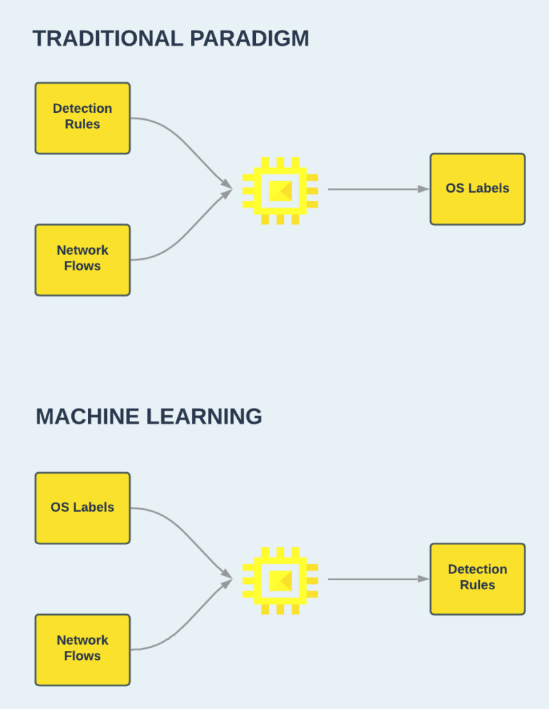
Figure 1: A traditional paradigm for writing identification rules vs. a machine learning approach. 

In the following sections, we will demonstrate how an ML model that generates OS identification rules can be created using a Decision Tree. A decision tree is a good choice for our task for a couple of reasons. Firstly, it is suitable for multiclass classification problems, such as OS identification, where a flow can be produced from various OS types (Windows, Linux, iOS, Android, Linux, and more). But perhaps even more importantly, after being trained, the resulting model can be easily converted to a set of decision rules, with the following form: 

if condition1 and condition 2 … and condition n then label 

 This means that your model can be deployed on environments with minimal dependencies and strict performance limits, which are common requirements for network appliances such as packet filtering firewalls and deep packet inspection (DPI) intrusion prevention systems (IPS). 

How do decision trees work for classification tasks?  

In this section we will use the following example dataset to explain the theory behind decision trees. The dataset represents the task of classifying OSs based on TCP/IP features. It contains 8 samples in total, captured from 3 different OSs: Linux, Mac, and Windows. From each capture, 3 elements were extracted: IP initial time-to-live (ITTL), TCP maximum segment size (MSS), and TCP window size.  

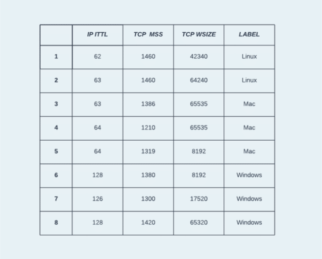
Figure 2: The training dataset with 8 samples, 3 features, and 3 classes. 

Decision trees, as their name implies, use a tree-based structure to perform classification. Each node in the root and internal tree levels represents a condition used to split the data samples and move them down the tree. The nodes at the bottom level, also called leaves, represent the classification type. This way, the data samples are classified by traversing the tree paths until they reach a leaf node. In Figure 3, we can observe a decision tree created from our dataset. The first level of the tree splits our data samples based on the “IP ITTL” feature. Samples with a value higher than 96 are classified as a Windows OS, while the rest traverse down the tree to the second level decision split. 

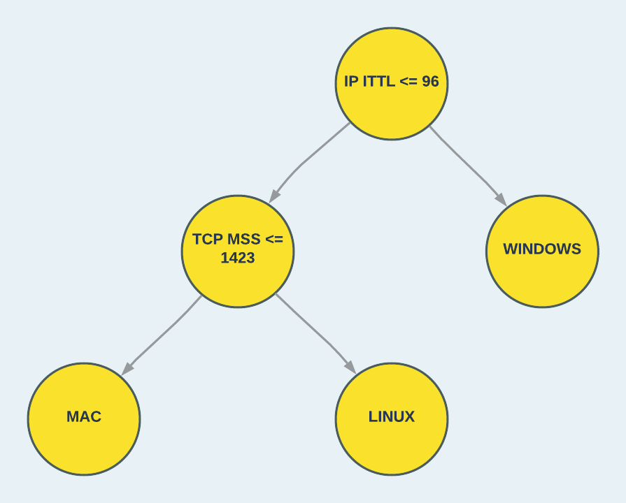
Figure 3: A simple decision tree for classifying an OS. 

So, how did we create this tree from our data? Well, this is the process of learning that was mentioned earlier. Several variations exist for training a decision tree; In our example, we will apply the well-known Classification and Regression Tree (CART) algorithm. 

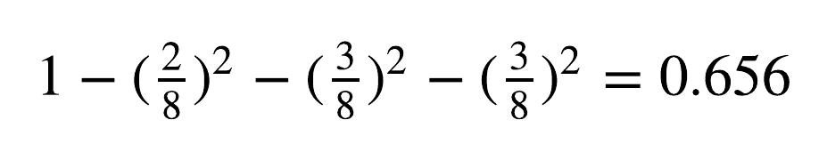
The process of building the tree is done from top to bottom, starting from the root node. In each step, a split criterion is selected with the feature and threshold that provide the best “split quality” for the data in the current node. In general, split criterions that divide the data into groups with more homogeneous class representation (i.e., higher purity) are considered to have a better split quality. The CART algorithm measures the split quality using a metric called Gini Impurity. Formally, the metric is defined as: 

Where 𝐶 denotes the number of classes in the data (in our case, 3), and 𝑝 denotes the probability for that class, given the data in the current node. The metric is bounded between 0 and 1 the represent the degree of node impurity. The quality of the split criterion is then defined by the weighted sum of the Gini Impurity values of the nodes below. Finally, the split criterion that gives to lowest weighted sum of the Gini Impurities for the bottom nodes is selected.  

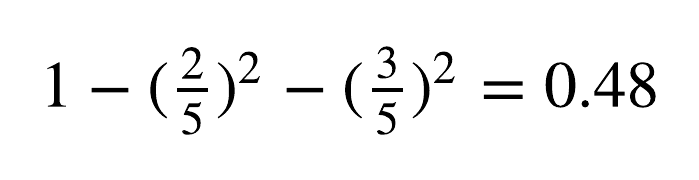
In Figure 4, we can see an example for selecting the first split criterion of the tree. The root node of tree, containing all data samples, has the Gini Impurity values of: 

Then, given the split criterion of “IP ITTL <= 96”, the data is split to two nodes. The node that satisfies the condition (left side), has the Gini Impurity values of:   

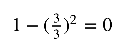
While the node that doesn’t, has the Gini Impurity values of: 

Overall, the weighted sum for this split is: 

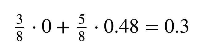
This value is the minimal Gini Impurity of all the candidates and is therefore selected for the first split of the tree. For numeric features, the CART algorithm selects the candidates as all the midpoints between sequential values from different classes, when sorted by value. For example, when looking at the sorted “IP ITTL” feature in the dataset, the split criterion is the midpoint between IP ITTL = 64, which belongs to a Mac sample, and IP ITTL = 128, which belongs to a Windows sample. For the second split, the best split quality is given by the “TCP MSS” features, from the midpoint between TCP MSS = 1386, which belongs to a Mac sample, and TCP MSS = 1460, which belongs to a Linux sample. 

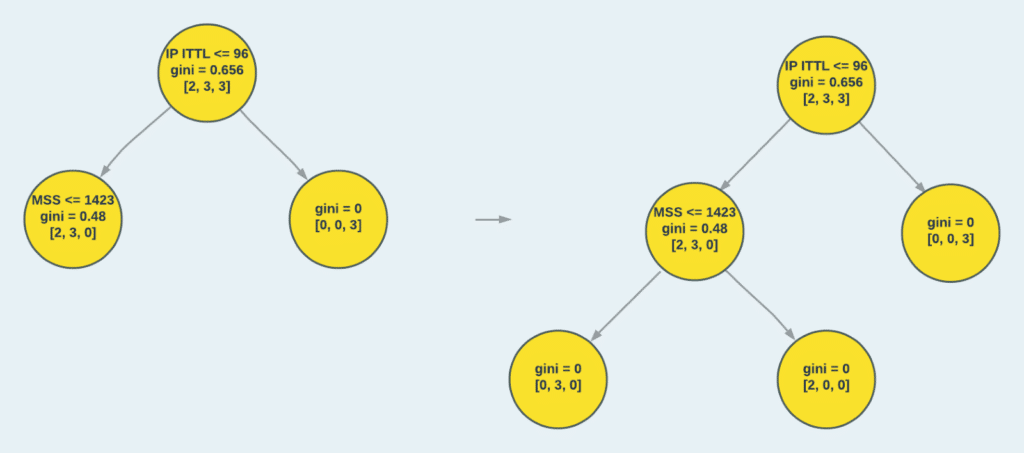
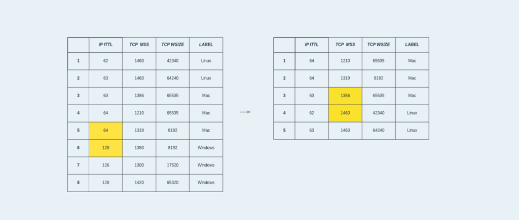
Figure 4: Building a tree from the data – level 1 and level 2. The tree nodes display: 1. Split criterion, 2. Gini Impurity value, 3. Number of data sample from each class. 

In our example, we fully grow our tree until all the leaves have a homogenous class representation, i.e., each leaf has data samples from a single class only. In practice, when fitting a decision tree to data, a stopping criterion is selected to make sure the model doesn’t overfit the data. These criteria include maximum tree height, minimum data samples for a node to be considered a leaf, maximum number of leaves, and more. In case the stopping criterion is reached, and the leaf doesn’t have a homogeneous class representation, the majority class can be used for classification.  

Everything You Wanted To Know About AI Security But Were Afraid To Ask | Watch the Webinar

From tree to decision rules 

The process of converting a tree to rules is straight forward. Each route in the tree from root to leaf node is a decision rule composed from a conjunction of statements. I.e., If a new data sample satisfies all of statements in the path it is classified with the corresponding label.  

Based on the full binary tree theorem, for a binary tree with 𝑛 nodes, the number of extracted decision rules is (𝑛+1)/ 2. In Figure 5, we can see how the trained decision tree with 5 nodes, is converted to 3 rules.  

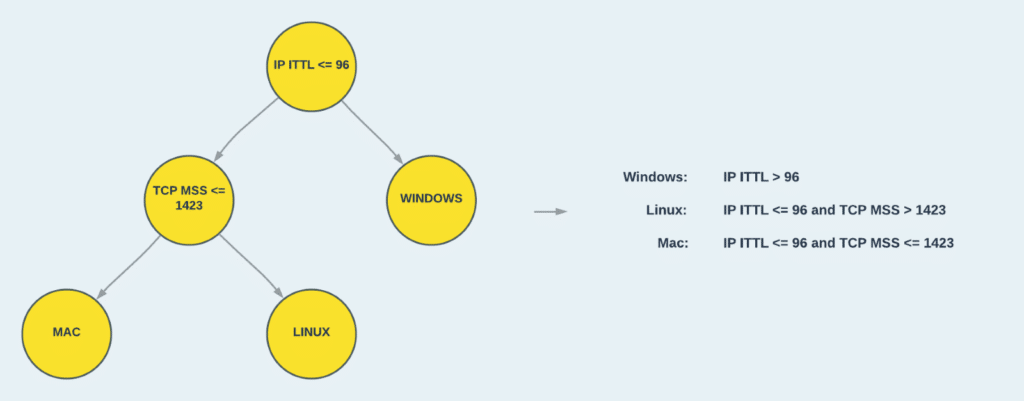
Figure 5: Converting the tree to a set of decision rules. 

Cato’s OS detection model 

Cato’s OS detection engine, running in real-time on our cloud, is enhanced by rules generated by a decision tree ML model, based on the concepts we described in this post. In practice, to gain a robust and accurate model we trained our model on over 10k unique labeled TCP SYN packets from various types of devices. Once the initial model is trained it also becomes straightforward to re-train it on samples from new operating systems or when an existing networking implementation changes. 

We also added additional network features and extended our target classes to include embedded and mobile OSs such as iOS and Android. This resulted in a much more complex tree that generated 125 different OS detection rules. The resulting set of rules that were generated through this process would simply not have been feasible to achieve using a manual work process. This greatly emphasizes the strength of the ML approach, both the large scope of rules we were able to generate and saving a great deal of engineering time. 

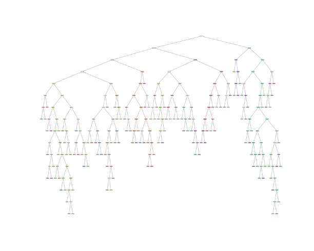
Figure 6: Cato’s OS detection tree model. 15 levels, 249 nodes, and 125 OS detection rules. 

Having a data-driven OS detection engine enables us to keep up with the continuously evolving landscape of network-connected enterprise devices, including IoT and BYOD (bring your own device). This capability is leveraged across many of our security and networking capabilities, such as identifying and analyzing security incidents using OS information, enforcing OS-based connection policies, and improving visibility into the array of devices visible in the network. 

An example of the usage of the latter implementation of our OS model can be demonstrated in Figure 7, the view of Device Inventory, a new feature giving administrators a full view of all network connected devices, from workstations to printers and smartwatches. With the ability to filter and search through the entire inventory. Devices can be aggregated by different categories, such as OS shown below or by the device type, manufacturer, etc. 
 

Figure 7: Device Inventory, filtering by OS using data classified using our models

However, when inspecting device traffic, there is other significant information besides OS we can extract using data-driven methods. When enforcing security policies, it is also critical to learn the device hardware, model, installed application, and running services. But we’ll leave that for another post. 

Wrapping up 

In this post, we’ve discussed how to generate OS identification rules using a data-driven ML approach. We’ve also introduced the Decision Tree algorithm for deployment considerations on minimal dependencies and strict performance limits environments, which are common requirements for network appliances. Combined with the manual fingerprinting we’ve seen in the previous post; this series provides an overview of the current best practices for OS identification based on network protocols.