How to Improve Elasticsearch Performance by 20x for Multitenant, Real-Time Architectures

Listen to post: Getting your Trinity Audio player ready...

A bit more than a year ago, Cato introduced, Instant*Insight (also called “Event Discovery”) to the Cato Secure Access Service Edge (SASE) platform. Instant*Insight are SIEM-like capabilities that improve our customers’ visibility and investigation capabilities into their Cato account. They can now mine millions of events for insights, returning the results to their console in under a second.

In short, Instant*Insight provides developers with a textbook example for how to develop a high-performance real-time, multitenant Elasticsearch (ES) cluster architecture. More specifically, once Instant*Insight was finished, we had improved ES performance by 20x, efficiency by 72%, and created a platform that could scale horizontally and vertically.

Here’s our story.

The Vision

To understand the challenge facing our development team, you first need to understand Instant*Insight and Cato. When we set out to develop Instant*Insight, we had this vision for a SIEM-like capability that would allow our customers to query and filter networking and security events instantly from across their global enterprise networks built on Cato Cloud, Cato’s SASE platform.

Customers rely on Cato Cloud to connect all enterprise network resources, including branch locations, the mobile workforce, and physical and cloud datacenters, into a global and secure, cloud-native network service that spans more than 60 PoPs worldwide. With all WAN and Internet traffic consolidated in the cloud, Cato applies a suite of security services to protect traffic at all times.

As part of this process, Cato logs all the connectivity, security, networking, and heath events across a customer’s network in a massive data warehouse. Instant*Insight was going to be the tool by which we allow our users to filter and query that data for improved problem diagnostics, planning, and more.

Instant*Insight needed to be a fully multitenant architecture that would meet several functional requirements:

• Scale — We needed a future-proof architecture that would easily scale to support Cato’s growth. This meant horizontal growth in terms of customer base and PoPs, and vertical growth in the continuously increasing number of networks and security events. Already, Cato tracks events with more than 60 different variable types for which there are more than 250 fields.
• Price — The design and build had to use a cost optimal architecture because this feature is being offered as part of Cato at no additional price to our customers. Storage had to be optimized as developing per customer storage was not an option. Machine power should also be utilized as much as possible.
• UX — The front-end had to be easy to use. IT professionals would need to see and investigate millions of events.
• Performance — Along with being usable, Instant*Insight would need to be responsive. It had to serve up raw and aggregated data in seconds. Such investigations are required to support queries for time periods such as a day, a month, or even a quarter.

The Architecture

To tackle these challenges, we sought to design a new, real-time index multitenant architecture from the bottom up. The architecture had to have an intuitive front-end user, storage that would be able to both index and serve tremendous amounts of data, and a back-end implementation that should be able to process real-time data while supporting high concurrency on sample and aggregation queries.

After some sketches and brainstorming, the team started working on the implementation. We decided to use Apache Storm to process the incoming metadata fed by the 60+ Cato PoPs across the globe. The data would be indexed by Elasticsearch (ES). ES queries would be generated at a Kibana-like interface and first validated by a lightweight backend. Let’s take a closer look.

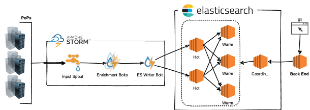
Apache Storm

As noted, Cato has 60+ PoPs located around the globe providing us with real-time, multitenant metadata. To keep up with the increasing pace of incoming data, we needed a real time processing system that could scale horizontally to accommodate additional events from new PoPs. Apache Storm was chosen for the task.

Storm is a highly scalable, distributed stream processing computation framework. With Storm, we can increase the number of sources (called “spouts” in Apache Storm) of incoming metadata and operations (called “bolts” in Apache Storm) that are performed at each processing step all of which can be eventually scaled on top of a cluster.

In this architecture, PoP metadata is transferred to a Storm cluster (using Storm spouts) via enrichment and aggregation bolts that eventually output events to an ES cluster and queueing alerts (emails) to be sent.

Enrichment bolts are a key part in making the UX responsive. Instead of enriching data when reading events (an expensive operation) from the ES cluster, we enrich the data at write time. This both saves query time and is better for using ES abilities to aggregate data (instead of enriching when querying from ES). The enrichment adds metadata that is taken from other sources such as our internal configurations database, IP2Location database, and merges more than ~250 fields to ~60 common fields for all event types.

ES Indexing, Search and Cluster Architecture

As one might assume, the ES cluster should continuously index and serve the events to Instant*Insight users on demand. This allows for real-time visibility of the SASE platform. It was clear from the beginning that we needed ES time-based indices and we started with the widely recommended hot — warm architecture. Such an approach optimizes hardware and machine types for their tasks. An index per day approach is an intuitive structure to choose with this architecture.

The types of AWS machine configurations that we chose were:

• Hot machines — These machines have optimal disks for fast paced indexing of large volumes of data. We chose AWS r5.2xlarge machines with io1 SSD EBS volumes.
• Warm machines — These machines provide large amounts of data that need to be optimized for throughput. We chose AWS r5.2xlarge machines with st1 HDD EBS volumes.

To achieve fast-paced indexing, we gave up on replicas during the indexing process. To avoid potentiation data loss, we put some effort on a proprietary recovery path in case of a hot machine failure. We only created replicas when we moved the data to warm machines. We achieved resiliency in-house, keeping the incoming metadata as long as the data is in a hot machine (~1-day old metadata) and was not replicated on the warm machines. This means that in case of a hot machine failure, we would have to re-index the lost data (events of 1 day).

Back-End

The Instant*Insight backend bridges between the ES cluster and the front-end. The back-end is a very lightweight stateless implementation that does a few simple tasks:

• Authorization enforcements to prevent non-authorized users from accessing data.
• Translation of front-end queries into ES’s Query DSL (Domain Specific Language).
• Recording traffic levels and performance for further UX improvements.

Front-End

For the front-end, we wanted to provide a Kibana-like discovery screen since it is intuitive and the unofficial UX standard for SIEMs. Initially, we checked if and how Kibana could be integrated into our management console. We soon realized that it would be easier to develop our own custom Kibana-like UX for several reasons. For one, we need our own security and permission protocols in place. Another reason is because fields on the side of our screen have different cardinality and aggregations from those in Kibana’s UX. Our aggregations show full aggregative data instead of counting the sample query results. Also, there are differences in requirements of a few minor features like the behavior that the histogram should be aligned across other places in our application.

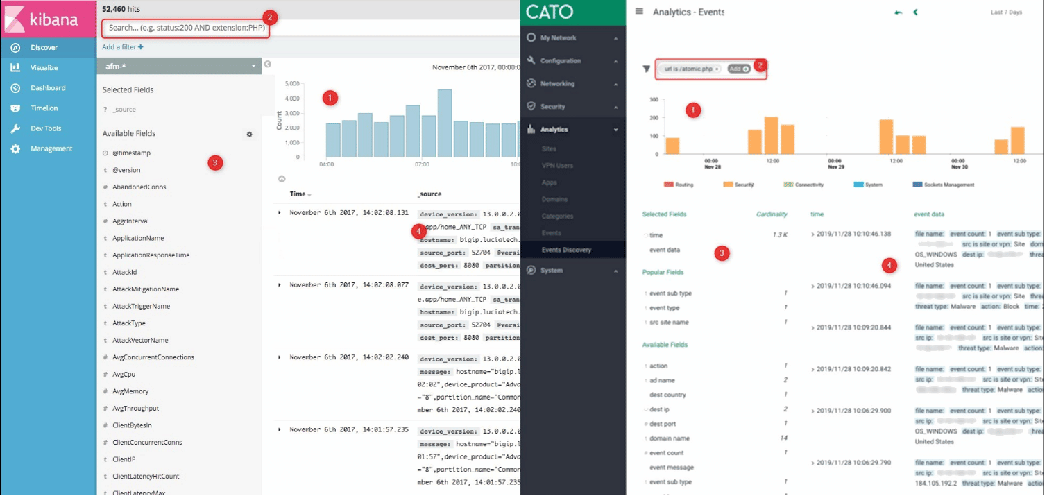
Development of the front end was not difficult, and within a few working days we had a functional SIEM screen that worked as expected on our staging environment. Ready to go to production, code was merged to master, and we started playing internally with our new amazing feature!

Not so surprisingly, the production environment tends to be a bit different from the staging one. Even though we performed some load and pressure tests on our staging during development, in production, a much greater data volume led the screen to behave worse and the user experience wasn’t as expected.

ES, UX and How They Interact

To understand what happened in production, one must better understand the UX requirements and behavior. When the screen loads, the Instant*Insight front-end should show the previous day’s events and aggregations for all fields for some tenant (Kibana Discover style). In this, the front-end performed well. But when we tried loading a few weeks’ worth of data, the screen could take more than a minute to render.

The default approach, having an index in ES comprised of multiple shards (self-contained Lucene indices), with each capable of storing data on all tenants, was found to be far from optimal. This is because requests were likely to be spread across the entire ES cluster. A one-month request, for example, requires fetching data from 30 daily indices multiplied by the number of shards in each index. Assuming there are 3 shards per index, 90 shards will need to be fetched (If we have less than 90 machines — it is the entire cluster). Such an approach is not only inefficient but also fails to capitalize on ES cache optimizations, which provide a considerable performance boost. Having an entire cluster that is busy with one tenant’s request obviously makes no sense. We had to change the way we index.

Developing a More Responsive UX and a Better Cluster Architecture

After further research on ES optimizations and more board sketches, we made some minor UX changes allowing users to operate on an initial batch of data while delivering additional data in the background. We also developed a new ES cluster architecture.

UX Changes

While the front-end had to be responsive, we understood that some delay was inevitable. There’s no avoiding the fact that ES needs time to return query results. To minimize the impact, we divided data queries into smaller requests, each causing different work to be done on the ES cluster.

For example, suppose a user requests event data from a given timeframe, say the past month. Previously, the entire operation would be processed by the cluster. Now, however, that operation is divided into four requests fulfilled according to optimum efficiency. The top 100 samples, the simplest request to fulfil is fulfilled first. In less than a second, users see the top 100 samples on their screens from which they can start working. Meanwhile, the next two requests — 60 fields cardinality and time histogram with groups for five different types of events — are processed in the background. The last one, field aggregations, is only queried when the user expands the field to reduce load on the cluster — there is no point fetching top usages of all fields we have while user will be interested on only few of them and this is one of the more expensive operation we have.

ES Cluster Architecture Improvements

To improve cluster performance, we needed to do two things — reduce the number of shards per search for maximum performance and improve cache usage. While the best approach would probably be to create a separate shard for each tenant, there is a memory footprint cost (~20 shards in a node for a 1GB heap). To minimize that impact, we first turned to a routing feature that lets us divide data within index shards by tenant. As a result, the number of queried shards is reduced to the number of queried indices. This way instead of fetching 90 shards to serve one month’s query, we would be able to fetch 30 shards, a massive improvement but one that would be less than optimal for anything less than 30 machines.

The next thing we did was to extend the indices’ duration with more shards without increasing (actually decreasing) the number of shards in the cluster. For example, we had a total amount of 21 shards (7 indices * 3 shards each) in the cluster for one week, by changing to weekly indices with 7 shards each, we end up with 1 weekly index) * 7 shards = 7 shards only for a week. A query of one month will now end up fetching 5 shards (in 5 indices) only, which requires a much smaller amount of computational power. One thing to note: querying a day’s data we’ll scan one-week of shards but since our users tend to fetch extended periods of data (weeks), it is very suitable for our use case (see Figure 3).

 

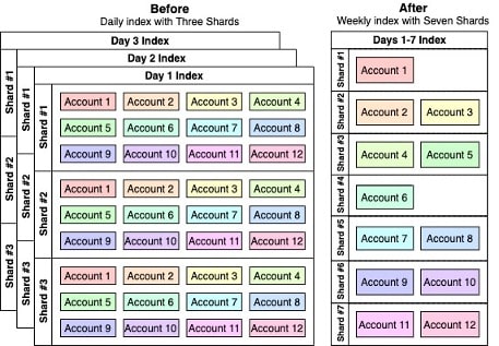
We need to find and measure the minimum number of shards that will provide the best performance given our requirements. Another powerful benefit of separating tenants into different shards is that it leads to better utilization of the ES cache. Instead of trying to fetch data from all shards, which constantly reloads the cache and degrades cluster performance, now we only need to fetch data from necessary shards, improving ES’s cache performance.

Addressing New Architecture Challenges

Optimizing the index structure for performance and improving the user experience, introduced new availability challenges. Our selected ES hot-warm architecture became less suitable for two reasons:

• Optimization of hot and warm machines from a hardware perspective is not a clear cut as before. Previously, “hot” machines performed most of the indexing and, as such, were optimized for network performance. The “warm” machines performed most of querying and, as such, were optimized for throughput. With the new approach, all machines are doing both functions — indexing and querying.
• Since we must index multiple days on the same index, our own recovery path is not a good option anymore because we’ll have to store data of days or weeks in-house. It will also be very hard to recover because of the amount of data we would need to re-index in the event of a failure.

As a result, the new architecture machines are now both indexing and handling queries while also writing replicas.

Performance Results

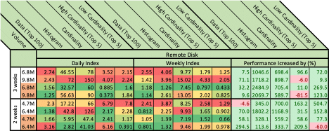
Results and details of the benchmarking we performed on real production data with respect to what is required from the UI behavior perspective can be found at the tables below. The benchmarking was always done when changing one parameter, what we called the “Measured Subject.” Each was evaluated by the time (in seconds) need to retrieve five types of measurement:

• Sample — A query for 100 sample results, which may be sorted and filtered per a user’s requirements.
• Histogram — A query for a histogram of events grouped by types.
• Cardinality — An amount of unique values of a field.
• High Cardinality (top 5) — The top 5 usages of a high cardinality field.
• Low Cardinality (top 5) — The top 5 usages of a low cardinality field.

While all queried information is important from a UX perspective, our focus is on allowing the user to start interacting and investigating as fast as possible. As such, our approach prioritized fulfilling sampling and histogram queries.

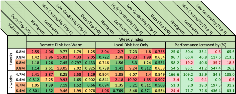
Below in Figures 4-6 are the detailed results. We define a “Measured Section” to be a measured subject with one of two period of times, two or three weeks. The volume column represents event amounts in millions. The orange cells in this column mark cached requests. Each of the figures represent one measured Subject. Each Subject is evaluated on two axes, for example, in figure 4 we compare daily index and weekly index performance while still using remote throughput optimized disks. Results are color coded from low response times (green) to high response times (red). Combining this information with the prior (cache-colored rows shown in orange) we can see how ES cache performs and (usually) improves performance. The “Diff” section compares the Measured Subjects. Those scores highlighted in green indicate that the Weekly Index is better; those scores highlighted in red indicate that the Daily Index is better. The numbers represent the percentage of increase in performance when moved from daily to weekly index. percent of change.

The first thing to do was to check how ES index structure (and routing) can impact performance. As can be seen in figure 4, the ES index structure gave a tremendous boost. For example, a histogram query for 3 weeks was reduced from 46.55 seconds to only 4.06, and with the cache in play, from 32.57 to only 1.26 seconds as can be seen on lines 1 and 3.

Both daily & weekly indices were tested running on the Hot-Warm architecture while having two Hot (r5.2xlarge + io1 SSD) machines and three Warm (r5.2xlarge + st1 HDD) machines. Understanding the big effect of how we index the events, we moved to benchmark other things. However, we will have to return to see if these are the most suitable index time frames and number of shards per index.

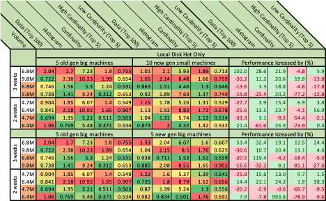
Next step was to check how moving from Hot-Warm architecture can impact performance. Running benchmarks led us to understand that even with lower throughput SSD disks, performance is still better when disks are local rather than remote. We’ve compared the previous Hot-Warm architecture to 5 Hot (i3.2xlarge) machines each having a local 1.9TB SSD. While performance is better, this still leads to another limitation to be considered: We can’t dynamically increase storage on machines.

 

So now knowing that local disks perform better, we had to select what kind of machines are the most suitable. The 10 new generation (I3en.xlarge) small machines with a 2.5TB local SSD didn’t perform better than the previous 5 (i3.2xlarge) machines.

Five new generation machines (I3en.2xlarge) with a 2×2.5TB local SSD didn’t perform any better than the previous 5 for the most valuable query (top 100 events). Remember, this query response allows the end-user to start working.

 

After defining our new architecture, we also benchmarked a different number of shards and time frames per index while making sure the number of total shards in the cluster will remain close between the benchmarks. We increased from one weekly index with seven shards to bi-weekly index with 14 shards, three weeks with 21 shards etc. (We added 7 shards for each week addition to an index.) Eventually, after checking a few different index time periods and shard amounts (up to a 1-month index) we found out that the (original) intuition of weekly index performed best for us and probably also the best with respect to our events retention policy (We need to be able to delete historical data with ease and weekly indices allows deletion of entire weeks.)

Conclusion

The measurements performed brought us to select a weekly index approach to be managed on top of i3.2xlarge machines with local 1.9TB NVMe SSDs. The table below shows how the changes impacted our ES cluster:

Metric / Index	First architecture	Second (improved) architecture
Index time range	Daily	Weekly
Shards in index	3	7
Total shards for year	1095 + replica = 2190	~365 + replica = ~730
Nodes	5 + coordinator	10 + coordinator
Shard Size	~4GB	Between 10GB and 20GB
Shards per node for year	219	~73

We dramatically decreased the amount of shards (by 3 times) while also increasing one shard size. Decreasing the amount of shards with more data in each one allows us to increase stored data at one node by up to 200% . (There is a limit of ~20 shards per 1GB of heap memory and we now have less shards with more data.). Bigger shards also improved overall performance in our multitenant environment because querying smaller number of shards for the same data as time range as before will release resources for next queries faster, queuing fewer operations. . Shard sizes varies because it depends on the number of events of the accounts it contains and unfortunately our control on how to route is very limited with ES. (ES decides by itself how to route between shards in index with some hash function on configured field.)

Since building the Instant*Insight feature, we already had to increase to 20 shards and added few machines to the cluster to accommodate expansions in the Cato network and increased the number of events. Responsiveness continues to be unchanged.

One should note that what is described in this article is the most suitable design for our needs; it might perform differently for your requirements. Still, we believe that what we have learned from the process can give some points of how to approach a design of ES cluster and what things are to be considered when doing so. For further information about optimizing ES design, read the Designing the Perfect Elasticsearch Cluster: the (almost) Definitive Guide.