Clustering-as-a-Tool: Leveraging Machine Learning for Device Data Insights and Signature Creation 

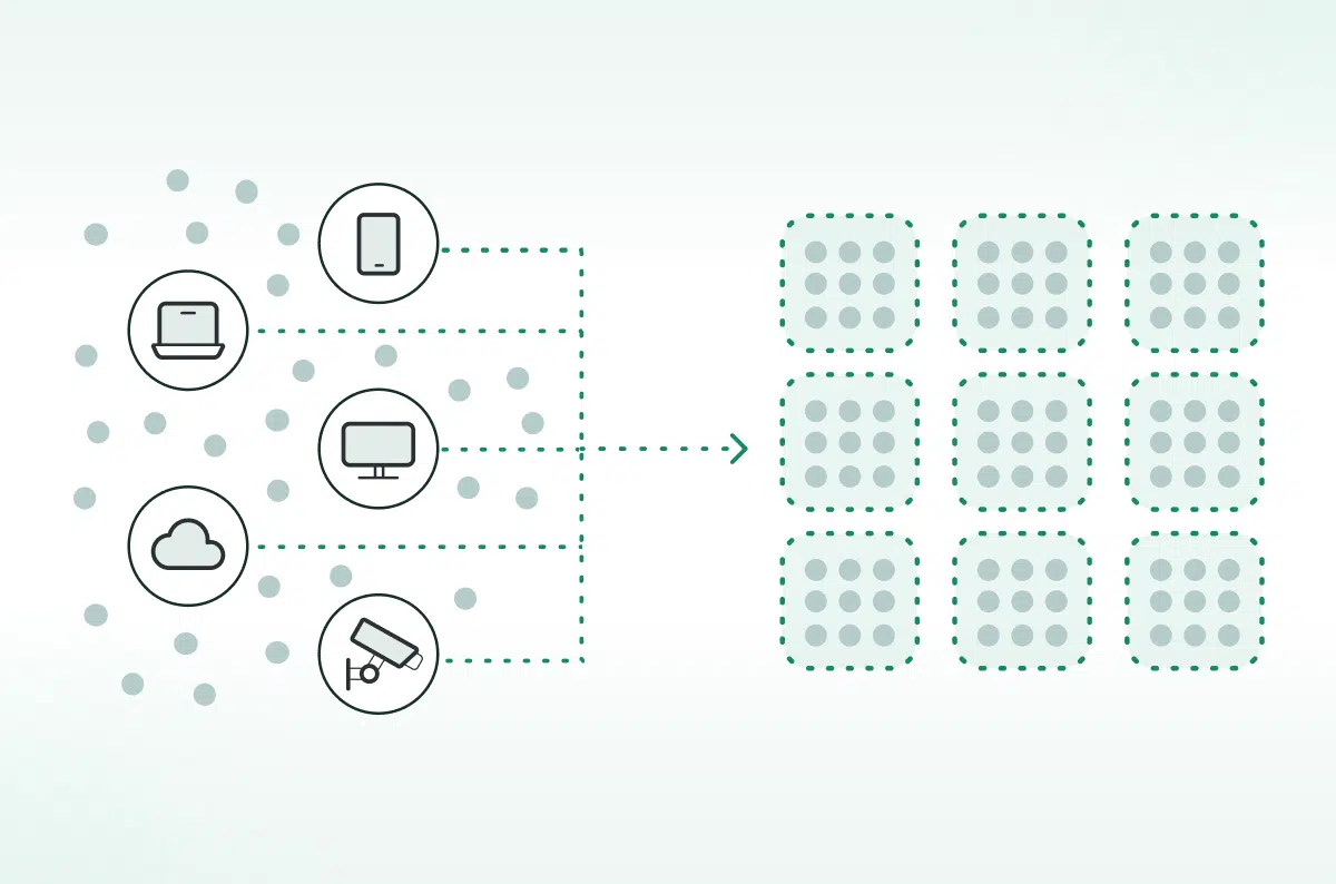
Imagine a retail chain, CaaT Networkstore, that wants to run a marketing campaign targeting its in-store customers. To do that, they need to know what types of devices their customers are using. They could survey the users, but a better, more accurate approach is to look at their free Wi-Fi logs and count the types of devices customers are using to connect to the network. If the store is small, the solution is fairly trivial. But as  CaaT Networkstore scales, sorting and classifying data manually becomes impossible.  

This same challenge confronts many enterprises. The network provides a rich source of data for answering many business and security questions, but the surge of data from logs and applications to sensors and more makes answering those questions difficult.  

To address this challenge, our engineering team developed a clear, practical workflow, which we call Cluster-as-a-Tool (CaaT). While we implemented CaaT as an internal tool, any engineering team can apply CaaT to address many such use cases in their organizations.  

The Problem 

CaaT has particular applicability to answering security problems. The influx of unmanaged network-connected devices from smartphones and IP cameras to access points and printers poses significant risk. These devices often come with outdated firmware, legacy protocols, and vulnerabilities that weaken the organization’s overall security posture. They open the door to botnets, lateral movement, and data exfiltration. 

Identifying devices accurately and at scale is essential but challenging. Manual processes don’t scale. And many tools stop at basic classification, leaving security teams blind to device behavior and risk exposure.  

The Solution 

 CaaT is an internal machine learning-based workflow that clusters network traffic patterns to surface specific device types. While earlier efforts focused on classifying operating systems, this workflow goes deeper – enabling granular fingerprinting of device models, firmware versions, and usage patterns. 

CaaT automates the process of: 

• Cleaning raw network data 

• Measuring behavioral similarity across devices 

• Clustering similar devices for classification 

• Visualizing and interpreting results interactively 

Instead of producing static classification rules, CaaT is used dynamically across different datasets and use cases. This approach helps data scientists and security teams iterate faster, uncover hidden devices, and enrich policy enforcement with greater confidence and precision. 

By integrating CaaT’s insights with broader network analytics, we can detect unmanaged or risky IoT devices in real time, enforce access controls, and proactively reduce the attack surface across the enterprise. 

First Example: Device Name Clustering 

To illustrate the workflow, let’s go back to the challenge facing  CaaT Networkstore.  Instead of surveying their users, they want to review the data collected as data streams through their access points.  Here’s a glimpse of what our dataset might look like: 

After collecting many more device names, we would have a problem: We lack a standard, unique device name. Some names are “Anner’s iPhone 14 Pro,” and another might be “Jack’s iPhone 14 Pro.” So, how do you easily aggregate them to identify that the iPhone 14 Pro is the most common device in the list? 

Intuitively, both names are very similar, as both contain “iPhone 14 Pro.” Therefore, searching for all names containing this value might yield all iPhone 14 Pro devices. But this is not scalable, as it requires us to know ahead of time what to search for, and there could be hundreds of different devices. To tackle that, we need to first find a deterministic metric that answers the question of, “How closely related are two different devices?” 

For this, we’ll use an edit-distance metric that counts the single-character edits required to transform one string into another.   

Tapping HDBSCAN to Provide Cluster Results  

Now that we have a list of device names and a distance function to compare them, we can determine similarity, but we lack a way to determine what degree of similarity actually puts them in the same class. To overcome that challenge, we move to the clustering phase using the HDBSCAN algorithm. 

The HDBSCAN algorithm works through seven steps: 

1. It identifies natural groups of points based on how close they are. 

2. It selects the most stable groups. 

3. It finds clusters of any shape instead of forcing round groups. 

4. It handles clusters of very different sizes without presetting a number. 

5. It automatically leaves outliers ungrouped. 

6. It doesn’t require heavy parameter tuning – we can guide it with two simple settings: 

• min_cluster_size: the smallest group accepted as a cluster. 

• min_samples: how strict it is about grouping points together. 

In our case, HDBSCAN groups device names that have a low distance metric and numerous enough, and marks device names without sufficiently similar matches as outliers. 

Interpreting Results Using UMAP Visualization 

We now have clustered results of the various phone names, but some clusters, though discrete, might share high similarity, such as “iPhone” and “iPhone 14 Pro.” To detect those similarities between clusters, we visualize our results using UMAP, an algorithm that projects high-dimensional data into two dimensions.  In the UMAP graphs, each cluster is a separate color.  Once the UMAP algorithm is done, HDBSCAN assigns cluster labels that we use to color those points, together producing a clear, intuitive map of device groupings: 

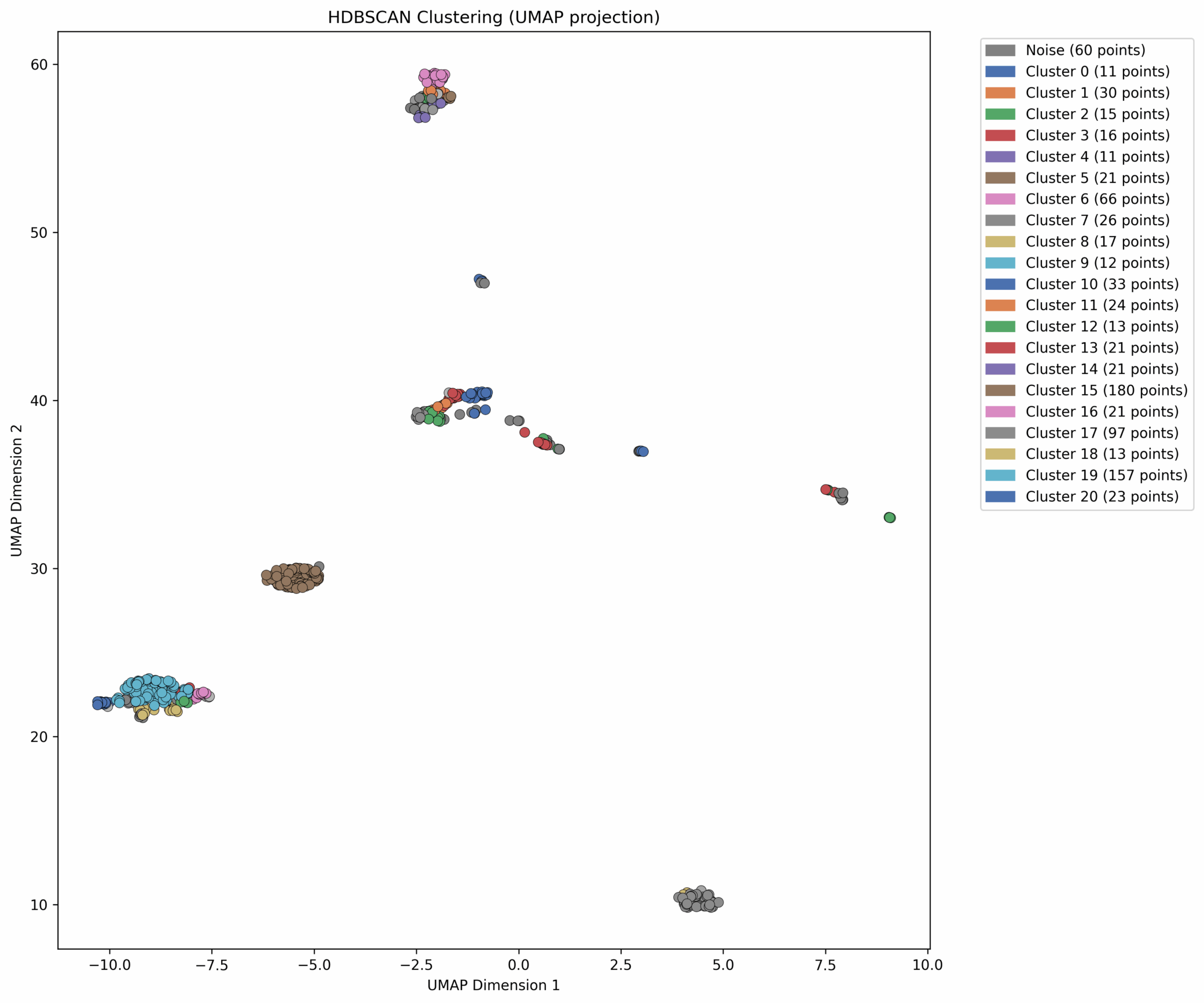
Figure 1. First example visualization 

The way we interpret this map is by asking ourselves, “Do the colors make sense?” Here, “make sense” means that we expect each tightly clustered group to have a single color. 

Following this logic, let’s zoom in on the points near the lower left. Cluster 19, the second-largest group, has several smaller clusters around it – are these different device versions of the same model? 

Tuning the Clustering Process 

In order to zero in on the most meaningful device families, we could turn clusters stricter or looser – by tweaking HDBSCAN’s parameters (min_cluster_size and min_samples), guided by our dataset’s size, our expectations, and the latest clustering results. 

 This tweaking process involves balancing clusters that are too wide and incoherent against clusters that are too small to properly represent a device family. For example, lowering min_samples makes clusters looser and might include the blob of points near Cluster 19 in the cluster. Striking that balance can make the next steps easier, although we won’t adjust it this time  

Collecting Insights 

Going back to where we started, CaaT Networkstore wants to know what the most used devices by their customers are, for the upcoming marketing campaign. Now we can answer this easily by reviewing a few device names from each of the larger clusters. 

For example, in cluster 19 we see both “Anner’s iPhone 14 Pro” and “Dave’s iPhone 14 Pro”, so we can safely conclude this cluster represents iPhone 14 Pro devices, meaning it’s one of the top devices used by our customers. All that’s left is to start working on the campaign! 

Second Example: Mixed-Indicator Clustering 

Let’s look at a trickier scenario: Suppose our retail chain, CaaT Networkstore, wants to improve its security posture, by creating a Firewall rule restricting IP cameras access to the internet. A prerequisite to it is identifying all IP cameras. This time, relying only on device names isn’t enough, so now we need to analyze other indicators, such as accessed domains, user-agents, etc. 

CaaT Networkstore could’ve just collected those devices IP addresses and used it in the Firewall rule, but this approach requires heavy maintenance and to make matters worse, the chain just acquired NimblePAN, a kitchenware shop – bringing in a wave of new, unclassified devices, with possibly many more unknown IP cameras. 

Even though this may seem complex, our workflow stays the same: we define a distance function between two devices and feed it into the HDBSCAN clustering algorithm. 

Let’s go through the workflow, redefine the distance between devices across multiple indicators, and transform our unstructured device data into actionable clusters, starting with looking at a sample of our dataset: 

Figure 2. Network logs

Let’s go over our workflow, step by step. 

Preparing the data 

1. Identify unique devices: Group records by IP address. In the previous example, this stage wasn’t necessary because we simply took device names, while this time we’ll have multiple data points related to the same device. The IP address works as a unifying key because every record, no matter what other details it carries, shares the same IP address when it’s from the same device. 

Aggregate counts: count the occurrences of each value and record the result in a single column, Instead of listing repeated entries. Let’s examine our devices to see what our data looks like after this stage: 

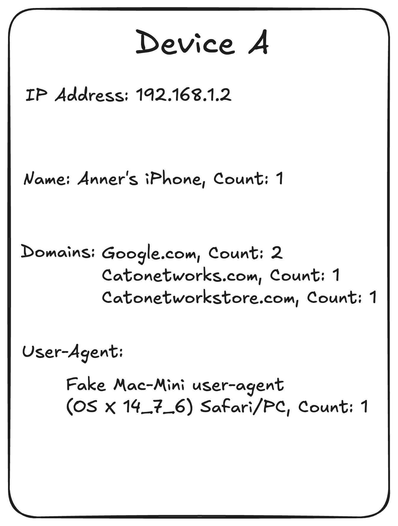
Figure 3. Device A

Figure 4. Device B

Normalizing Features & Computing Distances 

In order to be able to calculate the final distance which now depends on multiple features, we first need to compute each feature distance and normalize it – contrary to the first example, where only one feature was used. 

1. Device names: Use the same distance metric we referenced earlier. Calculating this distance for our two devices yields 7, as it takes seven edits to transform “Anner’s iPhone” into “Anner’s Mac Mini”. normalizing this distance is done by dividing by the length of the longer string – our maximum possible distance, so: 7 ÷ 17 ≈ 0.4. 
2. Domains: Intuitively, two devices accessing the exact same domains would be as similar as possible, meaning distance 0, while devices accessing completely different domains would’ve the furthest distance – 1. But what if there are three domains both devices access, and two domains that are unique to each device? Since each device can access many distinct domains, we will only take the top 5 domains it accessed and multi-hot encode them. We can use Jaccard Similarity – a fancy term that essentially means (in this case) the number of domains one device has that the other doesn’t, divided by the total distinct domains seen by either device. We calculate Jaccard distance by subtracting from 1 the number of bits that differ (popcount of XOR) divided by the number of bits set in either vector (popcount of OR). In the following visualization we compare our two devices. popcount equals the number of green bits, and we can compute the distance by calculating 1 – (2 ÷ 4) = 0.5.  

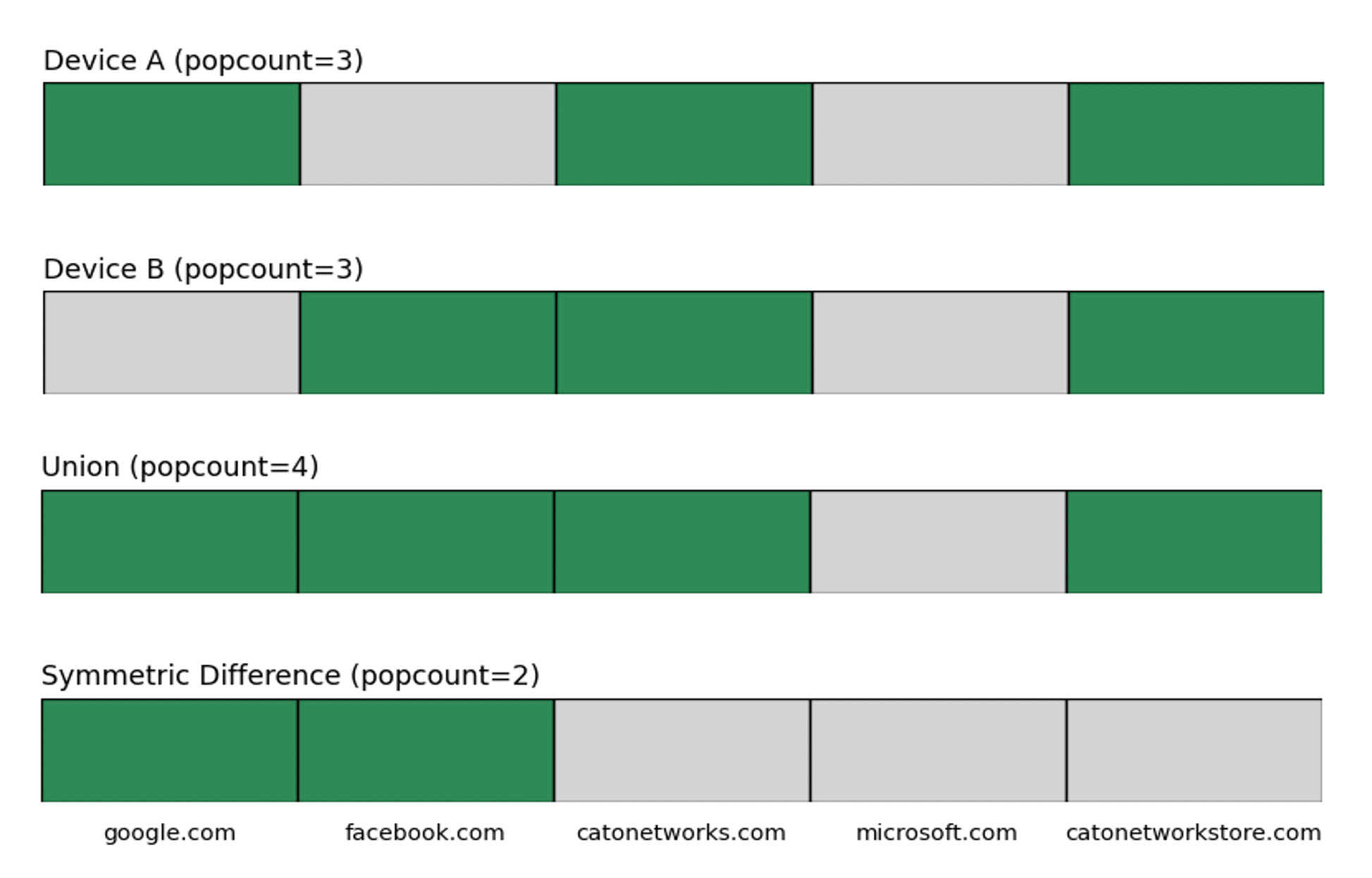
Figure 5. Domain distance calculation

3. User-agents: Similarity in user agents isn’t trivial, as even though there are known structures – they aren’t always used. Instead of comparing the entire string in the same manner of device name, we split each string into tokens and compare each one on his own. To amplify rarer token, weight is decided based on how rare a token is across the entire pool of user-agents. A near-perfect match means the two user-agents share almost all the same important words, while a poor match means they share very few. Because we’re also using weight, a good match can occur even if two user-agents don’t share many tokens, but those they do share are the rarer ones. Going back to our devices, we can see they share a few tokens: Fake, user-agent, and Safari. The rest of the tokens are unique to each device. Since all three shared tokens appear in many other user agents across our data, they carry little weight, whereas tokens like the version numbers (14_7_6, 17_7_2) are much rarer and receive extra weight. Taking all this into account gives a distance of about 0.9 between the two user agents. 

4. Define a composite metric: Gower distance allows us to average disparate measures into one score – and weight features (e.g. give device name matching twice the influence of domains) to reflect their importance (which we won’t do here, but is very useful). This is needed since currently each device is a precomputed string distances. This works by summing each feature’s result and dividing by the number of features: (0.4 + 0.90 + 0.50) ÷ 3 ≈ 0.60. Thus, the distance between device A and device B is 0.6, where 1 means completely different and 0 means identical. This indicates the devices are quite different – expected, since one is a mobile phone and the other is a PC.

Clustering & Visualizing 

1. Cluster with HDBSCAN: With every device as a numeric vector and a Gower-based distance function in hand, we feed it to HDBSCAN and let it uncover clusters automatically. 

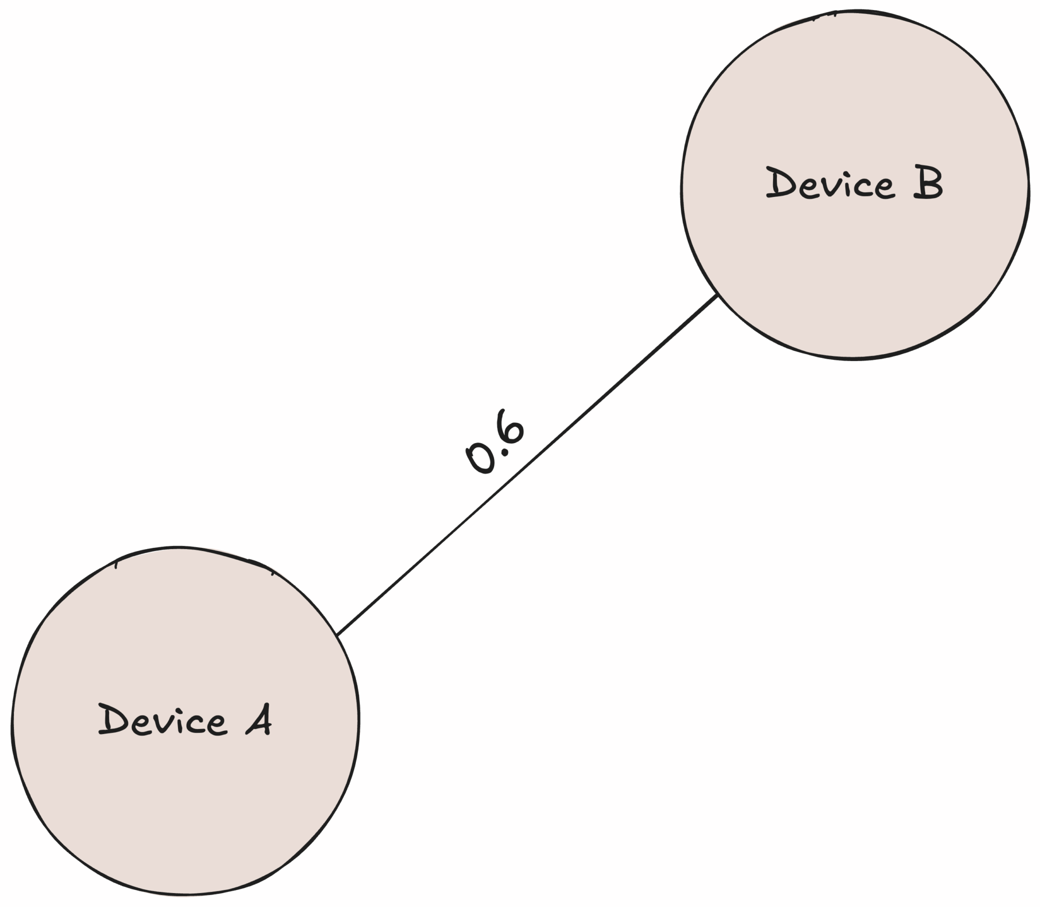
Figure 6. Final distance

2. UMAP projection: With HDBSCAN cluster labels in hand, we use UMAP to reduce the dimensions of the vectors to two dimensions and plot them on a map, coloring each point with its cluster label. 

Figure 7. Second example first visualization

Interpreting Results 

Unfortunately, our latest map doesn’t look quite right: some clusters are accurate, while others seem misplaced. For example, cluster 1 (the orange cluster) is split to two big clusters along with some extra points around it. At this point, we can tweak the HDBSCAN parameters and rerun our workflow, hoping to produce results that better pass our eye test.  

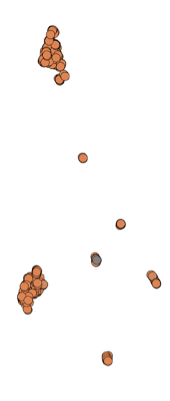
Figure 8. Misplaced cluster

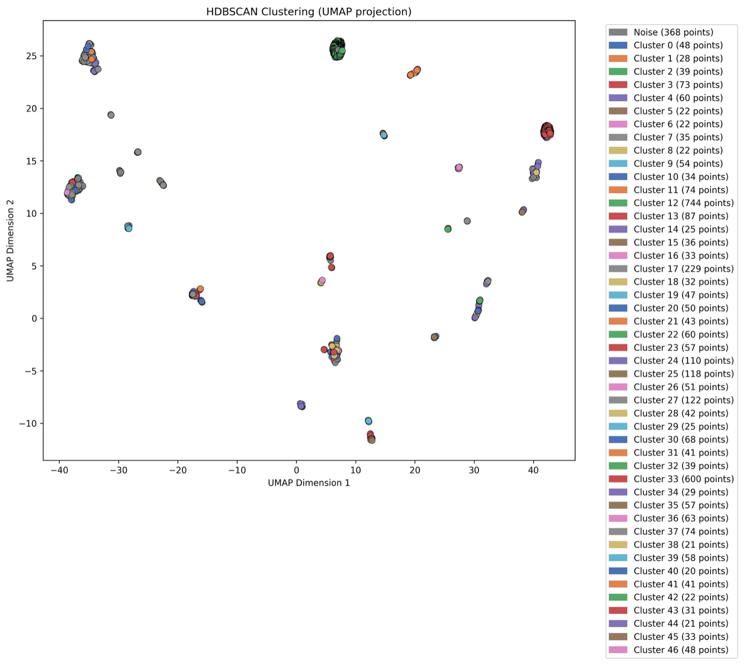
Figure 9. Second example second visualization

Notice how the point scatter stays the same, since the distances don’t change – but the cluster division changes, allowing for smaller, stricter clusters in this case. 

Also notice how clusters 12, 17, and 33 stayed large despite the tighter settings – that’s proof of how dense and coherent they are. Let’s dive into them. 

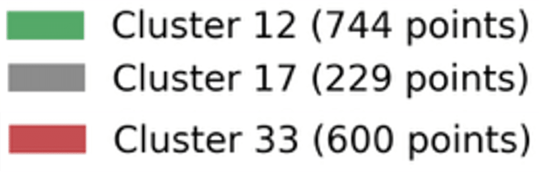
Figure 10. Three big clusters

• Cluster 12: Examining this cluster reveals that almost all devices have “iPhone” in their name and share a user agent similar to device A’s, with only slight version differences. 

• Cluster 17:  Devices in this cluster access variety of IP camera related domains and use user-agent strings that appear to be related to IP camera applications. Some devices in this cluster are even named ‘IPCAM’. 

• Cluster 33: This cluster contains devices with user agents closely related to device B’s but doesn’t always include the “Mac Mini” string, it also captures other model names. Since a secondary goal is to provide as specific a classification as possible, we could tweak our parameters to be stricter and rerun our workflow, or even create a new dataset derived from this cluster. 

Putting It All Together 

Going back to the main goal: CaaT Networkstore wants to write a Firewall rule restricting internet traffic from IP cameras. And as it turns out, we’ve just pinpointed those devices! Taking a second look at cluster 17 and at the indicators that caused those devices to be clustered together (device names, domains, user-agents), we now could tell if a certain device is an IP camera and write a firewall rule based on this predicate. 

Key Takeaways 

There are two major findings one can take from this work. FIrst, structured clustering cuts through the chaos. We are able to reveal natural device-type patterns by converting raw network data (or any data) into numeric vectors and clustering them. Automating this workflow in CaaT makes it even more comfortable and scalable. 

And second, experimentation is key. By interactively adjusting features, metrics, and clustering settings, and shifting between datasets – we gain deeper insights and uncover larger patterns in our data. This works because we treat clustering as a hands-on tool: human-guided tweaks, rather than fully automated steps, drive our exploration.